Logistic regression

In this post I will talk about one of the most basic models in Machine Learning: logistic regression. This post doesn’t assume any previous knowledge of logistic regression. Some prior knowledge on machine learning may be beneficial.

Introduction

Logistic regression is a machine learning model used to solve classification tasks. In a classification problem, we build a model that predicts the class label of an object, given its input features. In this post we will develop a model that predicts whether a board game is good or not given features like its complexity or number of players. Classification tasks like this, where the label has only two possible options, are called binary classification tasks. They are supervised learning problems.

Logistic regression is a generalized linear model. It is generalization of linear regression, which predictins an output variable as a linear combination of the input features (e.g. predicts the price of a house as a linear combination of its area, number of bedrooms…). It may be beneficial for the reader to have some knowledge on linear regression before reading this post, although it is not required.

In the following sections we will go through the basic maths behind logistic regression and work through an example of how to apply this model to binary classification.

Problem statement

Binary classification is the problem of predicting the class \(y \in \{0, 1\}\) of an object given a set of input features \(x \in \mathbb{R}^n\). To be able to train a model capable of making such predictions, we are given a set of correctly labeled examples: a set of points \((x^{(i)}, y^{(i)})\) with \(i \in [1, m]\).

As I am a big fan of board games, I will develop an example using this Kaggle dataset on board game data. The dataset comprises 5000 real boardgames, together with features as their number of players, average game duration, number of people that have bought the game, and so on. The games are ranked from best to not-as-good using a rating defined by this website. This Kaggle kernel contains the full code for the example we will develop. I will show some snippets here when relevant.

We will try to predict whether a board game is “top” or not, where we define a “top board game” as one being among the best 1000. Thus, \(y = 1\) if the game is one of the top 1000, and \(y = 0\) otherwise.

Our task is to build a model to predict y. For the sake of example, we will just use the two most relevant input features, as this will allow us to visualize the results better:

• \(x_1\) will be the number of buyers (owned in our dataset). As it seems logical, there is a strong positive correlation between the rating and the number of buyers: popular games are generally bought by more people than other games.
• \(x_2\) will be weight, which measures how complex a game is, in a scale from 1.0 to 5.0. Games with higher weight have more complicated rules and more complex mechanics. There is a positive correlation between rating and weight (top-ranked games tend to be complex ones).

In this case, we have than the number of training examples m = 5000 and the number of features n = 2. Each example \(x^{(i)} \in \mathbb{R}^2\).

Making predictions

As every machine learning algorithm, logistic regression has a number of parameters that will be learnt during training. Knowing the parameters and the input features, the model is able to predict the output variable y. So what are the parameters of logistic regression and how can we use them to output predictions?

It turns out that logistic regression is a linear model. Similarly to what linear regression does, we will compute the following linear combination of the input features for each example in the training set:

Where \(\theta_0\), \(\theta_1\) and \(\theta_2\) are the parameters of the logistic regression model.

However, z cannot be the output of our model, since we need to obtain a binary label, and \(z \in \mathbb{R}\). To obtain a prediction, we will apply the following function to z, known as the logistic or sigmoid function:

If we plot the function, we get the following shape:

• As we can see, \(y_{prob} \in (0, 1)\).
• Big negative values of z output values close to zero.
• Big positive values of z output values close to one.
• Inputs close to zero output values close to 0.5.

We can interpret this number as the probability that the given example belongs to the class \(y = 1\). So, if we perform this calculation for a certain example and obtain 0.1, that means that our model is convinced that this game is not top ranked. Conversely, if the had obtained 0.9, that would mean that our model is almost sure that the game is top ranked. We can take 0.5 as the boundary, such that we predict \(y = 0\) if \(y_{prob} < 0.5\), and y = 1 otherwise.

In the more general case, we have n input features. We can represent each example as a column vector of features \(x \in \mathbb{R}^n\). We can also define a column vector containing all the parameters in our model, \(\theta \in \mathbb{R}^n\). With this notation, we can write:

Training the model

As with every machine learning model, training a logistic regressor is just optimizing a cost function that tells the model how well it’s doing on the training set. For an individual training example (i), we will use the following function:

Where \(y^{(i)}\) are the real labels of the examples (often called the ground truths) and \(y_{prob}^{(i)}\) are the probabilities output by our model. This function is called the log loss function. It models our problem well because:

• If the actual label \(y^{(i)} = 0\), the first summand goes away, leaving the expression \(L(0, y_{prob}^{(i)}) = - log(1 - y_{prob})\), which is zero for \(y_{prob} = 0\) and tends to infinity for \(y_{prob} = 1\). Thus, if the actual label is zero, we are rewarding the model for outputing probabilities close to zero, and we are penalizing it for the opposite.
• If the actual label \(y^{(i)} = 1\), the second summand goes away, leaving the expression \(L(1, y_{prob}^{(i)}) = - log(y_{prob})\), which is zero for \(y_{prob} = 1\) and tends to infinity for \(y_{prob} = 0\) (the opposite to the previous bullet point).

This is for just one training example. The overall cost will be the average along all training examples:

We can see that this function depends on the model parameters \(\theta_0\) and \(\theta\), as the predictions \(y_{prob}\) are computed using these. Training the model becomes into an optimization problem: finding the parameters \(\theta_0\) and \(\theta\) that makes the cost function J as small as possible. We can employ algorithms such as gradient descent to solve this problem.

Example: the board game model

Let’s use sklearn Python library to train a logistic regression model for our board game problem. First of all, some imports:

1
2

from sklearn.linear_model import LogisticRegression
from sklearn.model_selection import train_test_split

We then load the data into a dataframe df. Our input features will be owned and weight, while the predicted variable will be top. I won’t show the code the read the data here. Feel free to check the Kaggle kernel if you are curious.

As usual in ML, we split our data into a train and a test set. We will use the first one to train the model, and the second one to evaluate its performance. We then fit our LogisticRegression object, which will solve the optimization problem described above:

1
2
3
4

X, y = df[['owned', 'weight']], df['top']
X_train, X_test, y_train, y_test = train_test_split(X, y, random_state=0)
model = LogisticRegression()
model.fit(X_train, y_train)

Alright, model trained. What are the value of the learned parameters? We can access them using:

1
2
3

theta0 = model.intercept_[0]  # theta0 = -5.76
theta1 = model.coef_[0][0]    # theta1 = 0.000726
theta2 = model.coef_[0][1]    # theta2 = 0.891

This means that, to make predictions, our model is computing:

The decision boundary

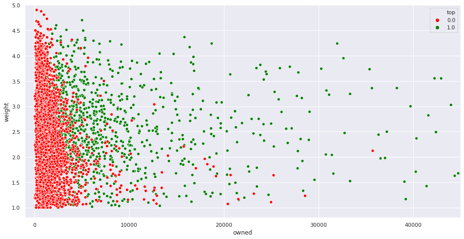
As we are just using two features for predictions, it is easy to visualize them. The following figure shows the two features in the two axes. Points in green represent top board games (\(y = 1\)), while points in red represent the other games (\(y = 0\)):

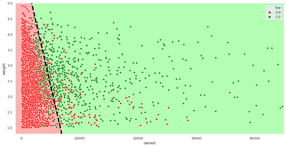
As you can see, points in the lower left corner are much more likely to have \(y = 0\) than points in the middle, for example. To make predictions, our model is going to split the feature space into two regions. Examples contained in the first region will be predicted as positive, with the other ones as negative. The decision boundary is the frontier between the two. As we are in \(\mathbb{R}^2\) and the model is linear, the decision boundary will be a straight line:

The dashed black line is the decision boundary. The points in the red region are classified as negatives and the ones in the green region, as positives.

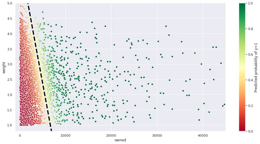
Let’s now visualize the predicted probability for each example.

Our model has a clear opinion on examples far away from the decision boundary. However, things get blurrier when we approach the dashed line, where \(y_{prob} = 0.5\).

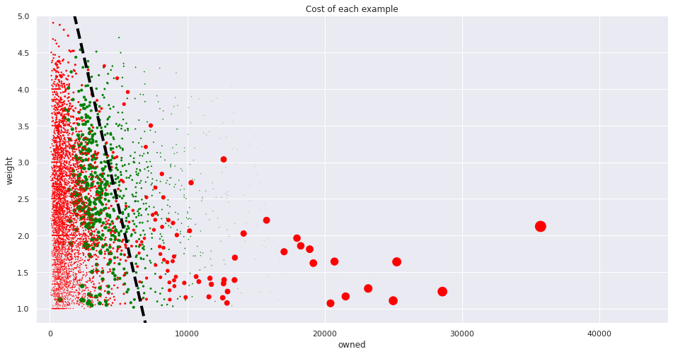
We talked earlier about the cost function, and how it penalizes the model making the wrong decisions. The following figure shows the cost associated to each example (the bigger the circle, the greater the cost):

As we mentioned earlier, misclassified examples are the ones incurring in greater cost. The further a misclassified point is from the decision boundary, the more sure our model is about making the wrong decision, and thus, the greater the cost. Fitting the model is equivalent to placing the dashed line in the position that minimizes the overall cost.

Evaluating the model performance

How good is our is our model at making predictions? Let’s use the test set to know it:

1

model.score(X_test, y_test) # Yields 0.9088

By default, LogisticRegression uses accuracy as evaluation metric. Accuracy is defined as:

That means that our model predicted 90.88% of the examples in the test set correctly. Not too bad for just using two features!

Conclusion

This finishes our study of logistic regression. I hope the example has helped to clarify some of the maths behind the model.

A couple final thoughts:

• For the sake of example, we have just considered two features. There are plenty of other variables to improve our model.
• The two employed features have very different scales. It may be beneficial for the model to normalize the variables, so they have a similar range and variance.
• Another term is usually added to the cost function presented here, called the regularization term, which helps prevent the overfitting problem. As this is not a concern in a model as simple as ours, we have omitted it here.
• We used accuracy for simplicity, but it may not be the best metric to choose, as the dataset is slightly imbalanced. Other metrics like ROC AUC or F1 score may be more adequate.

Hope you have liked the post! Feedback and suggestions are always welcome.

References

• Kaggle dataset on board game data: https://www.kaggle.com/mrpantherson/board-game-data.
• Insights - Geek Board Game (Kaggle kernel): https://www.kaggle.com/devisangeetha/insights-geek-board-game.
• Board Game Geek: https://boardgamegeek.com/.
• Machine Learning, Coursera course by Andrew Ng: https://www.coursera.org/learn/machine-learning/.
• Sklearn documentation: https://scikit-learn.org/stable/
• https://machinelearningmastery.com/types-of-classification-in-machine-learning/
• https://en.wikipedia.org/wiki/Supervised_learning