Some machine learning problems involve classifying an object into one of N classes. These are called multiclass classification problems, as opposed to binary classification, where there is just a positive and a negative class. Handwritten digit recognition and image classification are two well-known instances of multiclass classification problems.
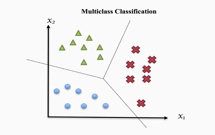
Image source: https://towardsdatascience.com/multi-class-classification-one-vs-all-one-vs-one-94daed32a87b
In this post we will explain how a neural network can be used to solve this problem. This is the second of a series of posts on neural networks I’ve been writing. If you are new to the topic, you may want to have a look into the first one before.
Problem statement
Let’s say we are working in an application for a factory processing fruits. Trucks bring oranges, lemons and limes mixed together. As a first step, a robot separates the fruits guided by a camera. Our task is to develop a model that classifies a fruit into one of the three groups given an input image. This is a multiclass classification problem with \(K = 3\) classes.
Each image can be translated into a set of input features \(x_1, x_2, ..., x_n\), with \(x_i \in \mathbb{R}\). A full discussion on the feature extraction process is beyond the scope of this post. As an option, we can understand the image as an array of numbers representing color intensities (one per pixel, for a grayscale image), and make each intensity an input feature. Other solutions may involve autoencoders and convolutional architectures.
Given an image’s features \(x_1, x_2, ..., x_n\), our model must predict a label \(y \in \{0, 1, 2\}\), with the following criteria:
\[\begin{matrix} y = 0 & \Rightarrow & Orange & \\ y = 1 & \Rightarrow & Lemon & \\ y = 2 & \Rightarrow & Lime & \\ \end{matrix}\]To train our model, we will have a collection of \(m\) correctly labeled images. We can represent these as a set of pairs \((x^{(i)}, y^{(i)})\), where \(x^{(i)} \in \mathbb{R}^n\) is the feature representation of the \(i\)th image, and \(y^{(i)} \in \{0, 1, 2\}\) tells us which fruit the image represents.
In the previous post we presented the following neural network, suitable for binary classification:
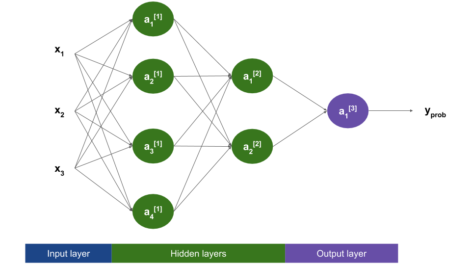
This network needs a couple changes before it can be used for multiclass classification. We will go over them in the next sections.
Label representation: one-hot encoding
The label representation \(y \in \{0, 1, 2\}\) may seem natural to us, but doesn’t work well for neural network training, as it implies an ordering between categories. By using this representation we are telling our network that \(Orange < Lemon < Lime\), which does not make any sense.
Instead, we will use a one-hot representation. With this scheme, our labels \(y\) become 3-dimensional vectors, with each element representing whether the fruit belongs to a certain class or not (i.e. the first element tells us whether the fruit is an orange or not, the second one whether it’s a lemon, and so on).
Using this representation, our training labels become:
\[\begin{matrix} y = \begin{bmatrix} 1 \\ 0 \\ 0 \end{bmatrix} & \Rightarrow & \text{Orange} \\ y = \begin{bmatrix} 0 \\ 1 \\ 0 \end{bmatrix} & \Rightarrow & \text{Lemon} \\ y = \begin{bmatrix} 0 \\ 0 \\ 1 \end{bmatrix} & \Rightarrow & \text{Lime} \\ \end{matrix}\]Note that classes are mutually exclusive: a fruit may be an orange or a lemon, but not both at the same time! This implies that exactly one element in the label vector must be one, with the other ones being zero. That’s why the encoding scheme is called one-hot!
In the general case, we will use vectors \(y \in \mathbb{R}^K\), with \(K\) being the number of classes. If an object belong to class \(c\), the vector’s \(c\)‘th element will be a one and the rest will be zero.
The output layer
In binary classification, the output layer produces a single value \(y_{prob}\), which we interpret as the probability of the object to belong to the positive class given the input features. This is coherent with labels, which are represented as a single value (0 or 1).
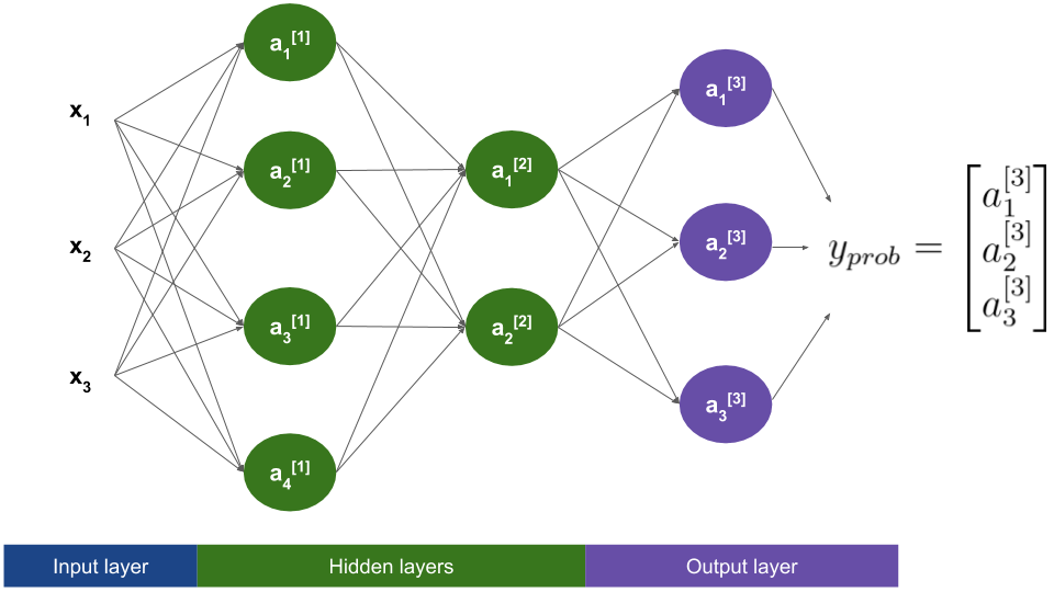
In multiclass classification we are using vectors of \(K\) elements as labels, instead. That means we will have to update our output layer to produce \(K\)-dimensional predictions. The new output vector \(y_{prob} \in \mathbb{R}^K\) will have as many numbers as possible classes. Each of these numbers will be between zero and one, and can be interpreted as the probability of the example to belong to each class. For example:
\[y_{prob} = \begin{bmatrix} 0.7 \\ 0.2 \\ 0.1 \end{bmatrix}\]This means that our networks thinks there is a 70% chance that the input picture is an orange, a 20% chance that it’s a lemon, and a 10% chance that it’s a lime. The final prediction would be orange. Note that all the probabilities in the output vector sum 1. This is required because the output labels are mutually exclusive: one picture can’t be an orange and a lemon at the same time.
So what’s the actual change? We will just increase the number of units in the output layer to three!
The activation function
In binary classification we used the sigmoid activation function for the output layer, as it guarantees that the output is between zero and one. Now that we have increased our output layer size, the sigmoid may not be the better choice. We could apply it independently to each output unit, but we would have no guarantee that the output probabilities add up to one, thus breaking our interpretation.
Instead, we will use the softmax activation function for the output layer. Given a vector \(\boldsymbol z \in \mathbb{R}^K\), the softmax function computes another vector of the same dimension, with its \(i\)th element being:
\[softmax(\boldsymbol z)[i] = \frac{e^{\boldsymbol z}[i]}{sum(e^{\boldsymbol z})} = \frac{e^{\boldsymbol z}[i]}{\sum_{c=0}^{K-1}e^{\boldsymbol z}[i]}\]Where \(e^{\boldsymbol z}\) is the exponential function, applied element-wise to the vector \(z\), and the square brackets indicate array indexing. Note that we are dividing by the sum of the exponentials. This guarantees that, if we add all the elements produced by the softmax, the result will be 1.0.
With these considerations, the output layer will do the following:
\[\boldsymbol z^{[3]} = \boldsymbol W^{[3]} \boldsymbol a^{[2]} + \boldsymbol b^{[3]}\] \[\boldsymbol a^{[3]} = y_{prob} = softmax(\boldsymbol z^{[3]})\]The matrix \(\boldsymbol W^{[3]}\) will have dimensions 3x2, thus guaranteeing that both \(\boldsymbol z^{[3]}\) and \(\boldsymbol a^{[3]}\) have as many elements as classes.
The loss function
For binary classification we can use the log loss (also called the cross-entropy loss), with the following formulation:
\[L(y, y_{prob}) = - y \ log(y_{prob}) - (1 - y) log(1 - y_{prob})\]Where \(y_{prob}\) is what our model predicted and \(y\) is the actual label. Recall that the loss function is defined for just one training example. To compute the total cost we would average over all the examples in our training set.
The form shown above is a particularization of the cross-entropy loss for two classes. For our example, we can use this generalization:
\[L(y, y_{prob}) = - y[0] \ log(y_{prob}[0]) - y[1] \ log(y_{prob}[1]) - y[2] \ log(y_{prob}[2])\]An example is worth a thousand words, so go through one. We will examine how the loss function behaves for three different predictions for the same image. Let’s say that we are given a picture of an orange. With our one-hot encoding strategy, the label would be:
\[\text{The example was an orange} \Rightarrow y = \begin{bmatrix} 1 \\ 0 \\ 0 \end{bmatrix}\]Case 1. The network works well for the example: it is 70% sure that what is saw was an orange.
\[y_{prob} = \begin{bmatrix} 0.7 \\ 0.2 \\ 0.1 \end{bmatrix}\] \[L(y, y_{prob}) = - 1 * log(0.7) - 0 * log(0.2) - 0 * log(0.1) = 0.3567\]Case 2. The network is unsure and thinks every fruit is equally likely.
\[y_{prob} = \begin{bmatrix} 0.33 \\ 0.33 \\ 0.33 \end{bmatrix}\] \[L(y, y_{prob}) = - 1 * log(0.33) - 0 * log(0.33) - 0 * log(0.33) = 1.1087\]Case 3. The network makes a mistake: it predicts a lime.
\[y_{prob} = \begin{bmatrix} 0.1 \\ 0.2 \\ 0.7 \end{bmatrix}\] \[L(y, y_{prob}) = - 1 * log(0.1) - 0 * log(0.2) - 0 * log(0.7) = 2.3026\]The loss function’s behaviour seems coherent:
- Case 1. If the network is confident about a prediction and it’s right, the cost is low.
- Case 2. If the network is uncertain, the cost is higher.
- Case 3. If the network is confident but the prediction ends up being wrong, the cost is the highest.
Also notice that the loss function only pays attention to the predicted probability of the actual class. In this example, the actual class was the first one, so the loss function only cares about the first element of \(y_{prob}\).
For the general case with \(K\) classes, the cross-entropy loss has the following formulation:
\[L(y, y_{prob}) = \sum_{c=0}^{K-1} - y[c] \ log(y_{prob}[c])\]If you want to dig deeper, this post explores the cross-entropy loss with multiple classes in depth.
Conclusion
That’s it! We now have all the elements in place to build a neural network that performs multiclass classification. We’ve covered the data format, the network architecture and the loss function. These are all the elements that we need to specify when creating a network using frameworks like Keras.
In the next post we will apply these concepts by using Keras to create and train a network to solve a classical handwritten digit recognition problem. See you soon!
References
- Deep Learning Specialization, Coursera courses by Andrew Ng: https://www.coursera.org/specializations/deep-learning
- Cross-entropy for classification, by Vlastimil Martinek: https://towardsdatascience.com/cross-entropy-for-classification-d98e7f974451
- Choosing the right Encoding method-Label vs OneHot Encoder, by Raheel Shaikh: https://towardsdatascience.com/choosing-the-right-encoding-method-label-vs-onehot-encoder-a4434493149b
- Multi-class Classification — One-vs-All & One-vs-One, by Amey Band: https://towardsdatascience.com/multi-class-classification-one-vs-all-one-vs-one-94daed32a87b