In this post I will talk about the underfitting and overfitting phenomena, and how model complexity affects them. I will also explain the bias-variance trade-off.
We will demonstrate these concepts with a binary classification example, where we will try to predict whether a forest elf will survive until being an adult or not based on two numeric features. This kernel contains the full code listing for this post.
This posts assumes that you know basic machine learning concepts like supervised learning or binary classification. We will use logistic regression as a model to demonstrate these concepts. If you are not familiar with it, you may check my other post on logistic regression. A basic faimiliarity with Python and sklearn is also necessary.
Model performance
Underfitting and overfitting are two phenomena that cause a model to perform poorly. But how do we define model performance? When working in any machine learning task, it is vital to define an evaluation metric that allows us to assess how good our model is.
We will be dealing with binary classification, so we will employ classification accuracy as a performance metric. Accuracy is defined as the ratio of correctly classified examples. It ranges between 0.0 and 1.0, and the higher, the better.
I will also use the term error throughout this post (as in “this model achieves a smaller error under these conditions”), meaning “the inverse of the performance metric”: the lower the metric, the higher the error.
Train and test set
To understand what over and underfitting is, we first need to explain the concept of train and test set.
Recall that in binary classification, we train our model on a collection of correctly labeled examples. This dataset is called the training set. After the model has been trained on this set, we can ask the model to make predictions on the examples in this dataset. Some of the examples will be classified correctly (most of them, hopefully), and some others won’t. We can thus calculate the error made by the model for this training set. This is called the training error.
However, doing well on the training set is not enough for a model to be good. We want our model to also do well on examples that hasn’t seen previously. In other words, we want our model to be able to generalize. The generalization error measures this capability.
The training error is not a good estimate for the generalization error, as it is based on examples the model has already seen. The model could “memorize” the training examples, achieving low training error, but fail to generalize. We will see later that this is called overfitting.
How can we obtain an unbiased estimation of the generalization error? Instead of using the entire labeled dataset to train the model, we will split it into two:
- The actual training set, used to train our model.
- The test set, used to evaluate the model’s performance.
After training the model, we will ask it to predict the classification labels for the examples in the test set. This will allow us to compute the test error, which is a better estimation of the generalization error.
An example
As promised, we will study how likely is a forest elf to surivive, given two physical features: height (which measures how tall the elf is) and ear_length (which should be obvious enough). We will try to predict whether the elf survives until being an adult or not.
As the savvy reader may have already realized, this is a made up dataset. It’s difficult to find real data that can show these concepts with just two features, which helps a lot with visualizations. The phenomena presented in this post are much more likely to happen in higher dimensional datasets.
Let’s visualize our dataset:
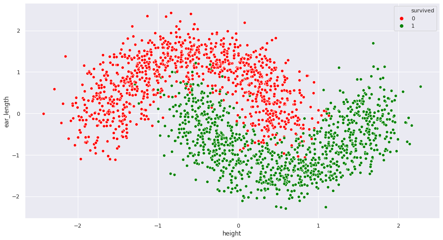
Some observations:
- It seems like there are heavy interactions between the two features. The variables are not independent.
- The features have been standardized: they have zero mean and similar dispersion. This will help us when creating polynomial features, in the next section.
- There is enough information to predict the class label using the two features. Negative examples are relatively grouped together, as positive examples are.
The dataset contains 2000 examples. Let’s split it into train and test, with leaving 75% in the training set and 25% in the test set. We will use sklearn’s train_test_split:
1
2
3
4
5
from sklearn.model_selection import train_test_split

df, y = ... # df contains the features, y contains the ground-true labels
X_train, X_test, y_train, y_test = train_test_split(df, y,
	test_size=0.25, random_state=0)
Note that sklearn will randomly shuffle the dataset before performing the split. Passing a constant as random_state ensures consistent results between runs.
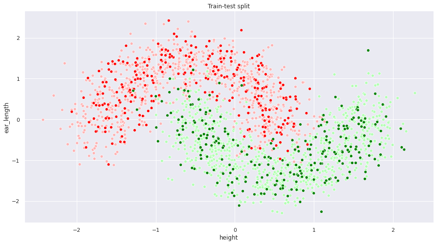
The following figure shows the aforementioned split. Lighter points belong to the training set, while darker ones have been assigned to the test set.
Underfitting
Let’s first build a plain logistic regression model and train it with our dataset (for an explanation about logistic regression, check out this post):
1
2
3
4
5
6
from sklearn.linear_model import LogisticRegression

model = LogisticRegression()
model.fit(X_train, y_train)
print(model.score(X_train, y_train))
print(model.score(X_test, y_test))
This model has an 86.9% accurancy on the training set and an 85.4% accuracy on the test set. That’s not optimal. Let’s visualize the decision boundary to get a feel of what is going on here:
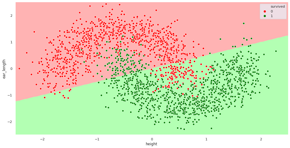
Our model is too simple to achieve a good performance on this dataset. Recall that logistic regression is a linear model. It is trying to separate the two classes using a straight line, which isn’t quite right. Both the train and the test errors are high. This situation is called underfitting.
Increasing model complexity: polynomial features
What can we do to make the situation better? We need to come up with a more complex model. One option would be to move away from logistic regression to a model that can learn non-linear decision boundaries by itself, like random forest or XGBoost. The other option is to make a more complex logistic regression model by adding polynomial features. This will be the approach to follow here.
Recall that, to make predictions, logistic regression is computing the following:
\[z = \theta_0 + \theta_1 x_1 + \theta_2 x_2\] \[y_{prob} = \sigma(z)\]Where \(\theta_i\) are the paremeters learnt by the model, \(x_0\) and \(x_1\) are our two input features and \(\sigma(z)\) is the sigmoid function. The output \(y_{prob}\) can be interpreted as a probability, thus predicting \(y = 1\) if \(y_{prob}\) is above a certain threshold (usually 0.5). Under these circumstances, it can be shown that the decision boundary is a straight line with the following equation:
\[\theta_0 + \theta_1 x_1 + \theta_2 x_2 = 0\]The problem here is that the decision boundary shouldn’t be a linear function of the two features, but should also contain:
- Higher-degree polynomial terms, e.g. \(x_0^2\), \(x_0^3\) and so on.
- Interaction terms, like \(x_0 x_1\) or \(x_0^2 x_1^3\).
Resulting in a model like this:
\[z = \theta_0 + \theta_1 x_1 + \theta_2 x_2 + \theta_3 x_1^2 + \theta_4 x_1 x_2 + \theta_5 x_2^2 + ...\] \[y_{prob} = \sigma(z)\]We can make logistic regression do this by manually creating polynomial features. We will create additional columns in the X_train and X_test matrices, containing the values of \(x_1^2\), \(x_2^2\), \(x_0 x_1\) and so on until a certain degree. We will feed these features to the model as if they were additional variables.
Sklearn has a built-in polynomial feature creator:
1
2
3
4
5
6
7
8
from sklearn.preprocessing import PolynomialFeatures

df, y = ... # df contains the features, y contains the ground-true labels
X = PolynomialFeatures(3).fit_transform(df)
X_train, X_test, y_train, y_test = train_test_split(df, y,
	test_size=0.25, random_state=0)
model = LogisticRegression()
model.fit(X_train, y_train)
With this code we get X to have the original features, as well as several additional columns: \(x_1^2\), \(x_1^3\), \(x_2^2\), \(x_2^3\), \(x_1 x_2\), \(x_1^2 x_2\) and \(x_1 x_2^2\). The first argument to PolynomialFeatures is the maximum degree of the polynomial features to create. It is important that \(x_1\) and \(x_2\) have a similar range of values. Otherwise, polynomial terms may end up being extremely high or low. Having our data standardized solves this problem.
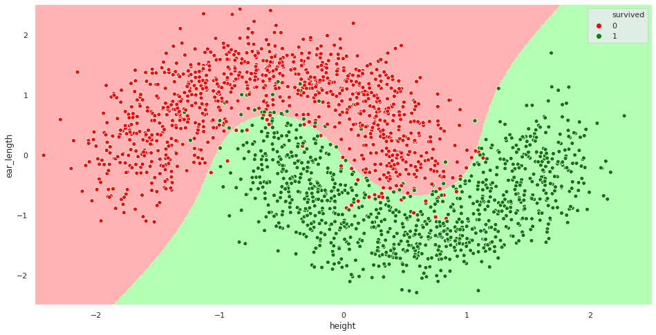
Fitting this model yields 96.7% accuracy on the training set and 95.4% on the training set. That’s much better! The decision boundary seems appropriate this time:
Overfitting
It seems like adding polynomial features helped the model performance. What happens if we use a very large degree polynomial? We will end up having an overfitting problem. Let’s see what happens when using a 15 degree polynomial (I’ve also turned regularization off, which increases the overfitting effect - we will talk about this later):
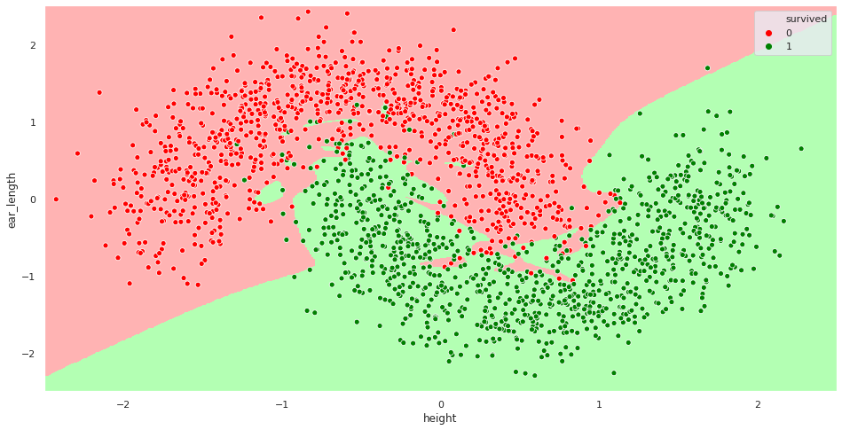
This model achieves a 98.9% accuracy on the training set, but drops to 93% on the test set. The model has so much flexibility that is fitting an over-complicated decision boundary that does not generalize well. It is memorizing the training set, which proves useless when facing the test set.
The bias-variance trade-off
As shown in the previous section, there is a trade-off in model complexity. Too complex models may overfit your data, while too simple ones are unable to represent it correctly. This trade-off between underfitting and overfitting is widely known as the bias-variance trade-off. But why is it called like that?
Bias and variance are two properties of statistical estimators:
- Bias estimates how far is the expected value of the estimator from the real value.
- Variance measures the dispersion of the estimator around its expected value.
In machine learning, we can decompose a model’s error in terms of these two properties:
- Bias tells us if the model is able to approximate the real underlying problem well. Our first model had high bias, as it was too simple to represent the dataset we were trying to classify. Having a high bias is thus a synonym of underfitting.
- Variance tells us how much the predictions would vary if the training set changed slightly. Our third model had high variance, as it was memorizing the training set. If we had trained the model on a slightly different training set, the model would have changed significantly. A model with high variance is thus overfitting the training set.
If you are interested in the mathematics underneath this decomposition, this post provides an in-depth explanation. The derivation is usually performed using the MSE loss function, common in regression. However, the bias and variance concepts are also applicable to classification, as we have seen.
As you saw in previous sections, changing the model complexity affects both bias and variance. More complex models tend to have higher variance and lower bias. On the other hand, simpler models will have lower variance but more bias. There is thus a trade-off between the two sources of error. To make a good model, we must balance the two terms wisely.
Factors affecting bias and variance
Bias and variance may be affected by several factors:
- As already explained, increasing model complexity (also called model capacity) increases variance and lowers bias. This applies not only to switching between models and adding polynomial features, but also to certain hyperparameters. For example, decision trees have a hyperparameter controlling the depth of the tree. The bigger the value, the bigger the tree and the more complex the model. Increasing this value will tend to decrease bias and increase variance.
- Adding more features tends to increase variance and decrease bias.
- Making the training set bigger (i.e. gathering more data) usually decreases variance. It doesn’t have much effect on bias.
- Regularization modifies the cost function to penalize complex models. Regularization makes variance smaller and bias higher. Sklearn’s
LogisticRegressionuses regularization by default. It can be disabled by settingpenalty='none', and its magnitude is controlled by theCparameter (the smaller, the greater regularization effect).
Diagnosing bias and variance problems
It is easy to diagnose if your model suffers from high bias or high variance when you have only two features by plotting them. But what happens if your dataset has more than two dimensions? Then you should look at the training set and test set errors.
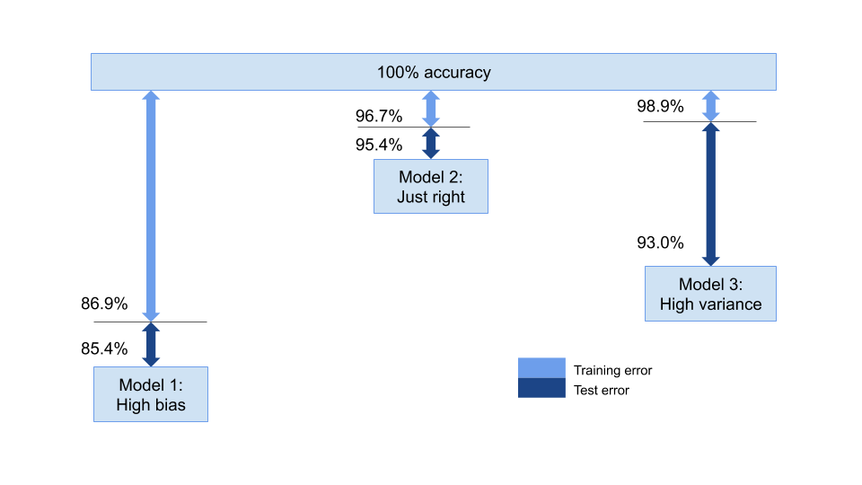
- If both the training set and test set errors are higher than what you would expect, it’s likely that you have a bias problem.
- If the training set error is very low but the test set error is not, then your model is failing to generalize, thus having a variance problem.
- If both errors are similar and as low as you would expect, then congratulations! Your model is just right.
The below diagram shows the three logistic regression models we’ve come up with in this post, together with their train and test errors:
Conclusion and further reading
Underfitting and overfitting, together with bias and variance, are very important concepts in machine learning. I hope this post helped you understand them better. You can also check this kernel if you’re interested in the programming details.
Some further thoughts:
- You may have seen people splitting datasets into three parts: a training set, a cross validation or dev set and a test set. Cross-validation is a technique for estimating model performance and tuning hyperparameters. You can read more about it here.
- We briefly talked about feature scaling and standardization. This post may provide further insights about these preprocessing techniques.
- Plotting learning curves is a technique to further diagnose if your model suffers from high bias or high variance. You can read this for further info.
Hope you have liked the post! Feedback and suggestions are always welcome.
References
- Machine Learning, Coursera course by Andrew Ng: https://www.coursera.org/learn/machine-learning/.
- 4 Types of Classification Tasks in Machine Learning, by Jason Brownlee: https://machinelearningmastery.com/types-of-classification-in-machine-learning/
- How to Use Polynomial Feature Transforms for Machine Learning, by Jason Brownlee: https://machinelearningmastery.com/polynomial-features-transforms-for-machine-learning/
- MSE and Bias-Variance decomposition, by Maksym Zavershynskyi: https://towardsdatascience.com/mse-and-bias-variance-decomposition-77449dd2ff55
- Holy Grail for Bias-Variance tradeoff, Overfitting & Underfitting, by Juhi Ramzai: https://towardsdatascience.com/holy-grail-for-bias-variance-tradeoff-overfitting-underfitting-7fad64ab5d76
- Scale, Standardize, or Normalize with Scikit-Learn, by Jeff Hale: https://towardsdatascience.com/scale-standardize-or-normalize-with-scikit-learn-6ccc7d176a02
- How to use Learning Curves to Diagnose Machine Learning Model Performance, by Jason Brownlee: https://machinelearningmastery.com/learning-curves-for-diagnosing-machine-learning-model-performance/
- Sklearn documentation: https://scikit-learn.org/stable/
- XGBoost documentation: https://xgboost.readthedocs.io/en/latest/