They are on everyone’s lips: every single post today seems to talk about deep neural networks and the bewildering variety of applications they are used for. Speech recognition, computer vision, natural language processing… the possibilities seem endless. Neural networks are the workhorse of deep learning, a subset of machine learning. But what is a neural network? How does it work?
This is the first of a series of posts on neural networks. Our ultimate goal will be to build a network able to recognize handwritten digits, as per the MNIST dataset. This first post presents what an artificial neural network is and the basic maths behind it. I’ve followed the same notation as Andrew Ng in his awesome Deep Learning specialization on Coursera.
To understand this post you should have basic notions of machine learning, linear algebra and calculus. In particular, you should already know what a classification problem is and how a logistic regression model can help. If you are not familiar with these concepts, this blog post may help. You should also know how to multiply matrices and what a derivative is.
Enough talk. Let’s dive deep into deep learning (pun intended)!
What is a neural network?
If you are super-hyped, expecting a definition that compares a neural network with human brain, you’re out of luck. A neural network is a machine learning model, just like logistic regression or XGBoost. Like these models, neural networks can be used for tasks like classification and regression.
What is the difference between traditional models and neural networks then? The latter are much more complex models. They may have billions of parameters, which allows them to learn really complex functions. This makes them suitable for incredible applications, like detecting objects (e.g. cars) in an image or diagnosing lung cancer given a radiography.
There are many types of neural networks depending on the field of application. Convolutional neural networks and recurrent neural networks are used in computer vision and natural language processing, respectively. In this post we will focus on artificial neural networks, often called fully connected networks or just neural networks, for short. These are the basic building block on which the others are based. It is important to understand these well before jumping into the others.
When to use a neural network
Before anyone gets too excited, a word of warning: as with every tool, it is adequate for some scenarios and it is not for other ones. If you try to apply neural networks to every single problem, chances are you will end up wasting your time.
Neural networks are complex models, and thus are adequate for complex problems (reading my post on model complexity may help understand). Applications like speech recognition, computer vision or natural language processing are usually the niche use for neural networks. If you have a simple classification problem with a couple plain numeric variables, chances are that XGBoost or random forest will work better.
As with any complex model, neural networks are prone to overfitting if you do not feed them with enough data. If you have very little data to solve your problem, neural networks aren’t likely to be very effective.
If you are interested, this post explores this topic in depth.
Logistic regression as a mini neural network
Let’s get ourhands dirty! How does a neural network work? How does it make predictions? It turns out that neural networks can be seen as a generalization of logistic regression. Let’s review the latter from a different angle before jumping into full-blown neural networks.
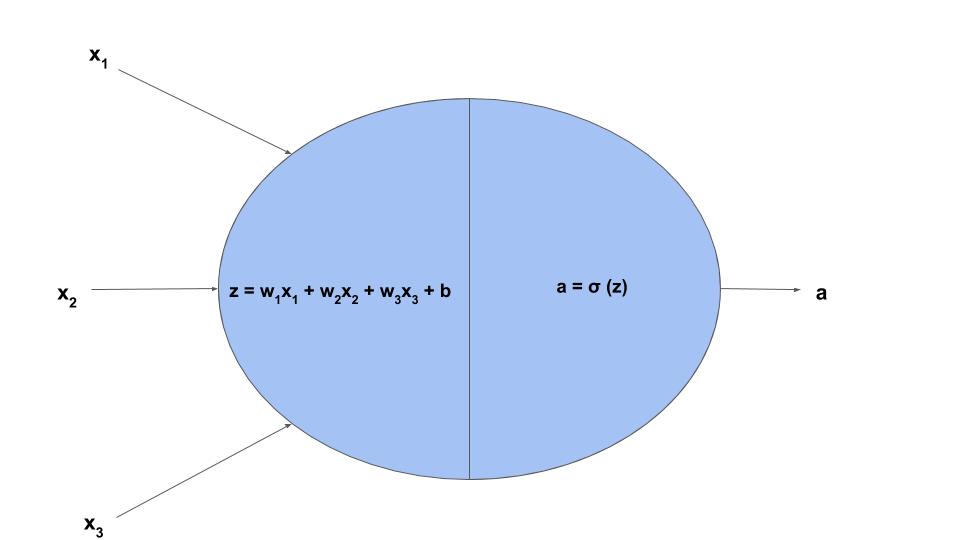
Let’s say we are trying to solve a binary classification problem using logistic regression (like this one). We are given the input features \(x_1, x_2... x_n\) and we are asked to predict the target label \(y \in \{0, 1\}\). This is what logistic regression would do:
- Compute a linear function of the inputs.
- Apply the sigmoid non-linear function to generate the prediction.
Where \(w_i\) are the weights of the logistic regression model and \(b\) is the bias term (if you read this, I called them \(\theta_i\) and \(\theta_0\), respectively). These are the parameters that the model learns by minimizing the cost function.
The sigmoid function makes the output have a non-linear relationship with the input. In the neural network context, these non-linear functions are called activation functions.
This simple logistic regression model can be thought of as a computation graph:

What does this have to do with neural networks? ANNs are composed of lots of units like the one shown above, interconnected to each other.
Anatomy of a neural network: layers
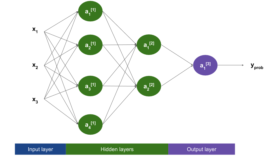
The idea of a neural network is to connect several units like the one above together, such that the output of one unit is wired to the input of another. Units are grouped in layers, forming a structure like the following:

Don’t get intimidated by the notation in this diagram! We will go through it in a minute.
As shown above, there are three types of layers:
- The input layer is shown in blue, and it is always the first one. It does no computation: it is just a way to represent the input to our network (the features \(x_i\)).
- The hidden layers, shown in green, perform the computation explained before: a linear function followed by a non-linear activation function. The first hidden layer gets the features as input, while deeper layers get the output of previous layer’s units.
- The output layer is the last one, and also performs a similar computation as hidden layers. For binary classification, the output layer has a single unit, and its result is the prediction of the network.
As the input layer does not perform any computation, we don’t count it as an actual layer. Thus, the above network has 3 layers. In general, a network may have \(L\) layers ( \(L = 3\) in this case).
Note that each unit is connected to every single unit in the previous layer. This is why this network architecture is sometime called fully connected.
The result of the computation performed by a unit is called the activation for that unit. In the next section we will see how these values are computed.
Computing activations
We will denote by \(a_i^{[l]}\) the activation of the \(i\)th unit in layer number \(l\). For example, \(a_3^{[1]}\) is the output of the 3rd unit of the first layer. Look at the figure in the previous section to double-check that you understand the notation. Thus, the text inside each unit repesents its output.
To compute the activations we must follow the same steps as in logistic regression. For the sake of example, let’s compute \(a_1^{[2]}\), the activation of the first unit in the second layer:
\[z_1^{[2]} = w_{21}^{[2]} a_1^{[1]} + w_{22}^{[2]} a_2^{[1]} + w_{23}^{[2]} a_3^{[1]} + w_{24}^{[2]} a_4^{[1]} + b_1^{[2]}\] \[a_1^{[2]} = g^{[2]}(z_1^{[2]}) = \sigma(z_1^{[2]})\]Wow, that seems intimidating. Don’t get fooled by this apparently complex expression: it is just the same as logistic regression! The only difference is that different units may have different values for the weights and the bias term. We are using the following notation:
- \(w_{ij}^{[l]}\) is the weight that unit \(j\) in layer \(l\) gives to the activation coming from the \(i\)th unit in the previous layer. In the diagram shown above, each arrow represents one of these weights. For example, the arrow going from \(a_2^{[1]}\) to \(a_3^{[2]}\) represents \(w_{23}^{[2]}\).
- \(b_{j}^{[l]}\) is the bias term for unit \(j\) in layer \(l\). They play the same role as \(b\) in logistic regression. They are not represented in the figure.
- \(g^{[l]}\) is the activation function for layer \(l\). For now, this is equivalent to the sigmoid function. We will see later that we can use other activation functions that work better than sigmoid for neural networks.
\(w_{ij}^{[l]}\) and \(b_{j}^{[l]}\) are the learnable paremeters of the neural network: they can be trained by minimizing a cost function, as in logistic regression.
Matrix notation
Do you like subscript notation? Neither I do. It turns out that all the computations in a neural network can be expressed as matrix operations. This simplifies notation a lot and makes implementations much faster, as computers prefer matrix operations to loops.
We can stack the \(z\) values and the activations in a single column vector per layer. If we do this, we get:
\[\boldsymbol z^{[l]} = \begin{bmatrix} z_1^{[l]} \\ z_2^{[l]} \\ ... \\ z_{n_l}^{[l]} \end{bmatrix} \text{ } \boldsymbol a^{[l]} = \begin{bmatrix} a_1^{[l]} \\ a_2^{[l]} \\ ... \\ a_{n_l}^{[l]} \end{bmatrix}\]\(n_l\) represents the number of hidden units in layer \(l\). In the network above, \(n_1 = 4\), \(n_2 = 2\) and \(n_3 = 1\). The vectors \(\boldsymbol z^{[l]}\) and \(\boldsymbol a^{[l]}\) have dimensions \((n_l, 1)\).
We can also stack the biases into a vector and the weights into a matrix, defining:
\[\boldsymbol b^{[l]} = \begin{bmatrix} b_1^{[l]} \\ b_2^{[l]} \\ ... \\ b_{n_l}^{[l]} \end{bmatrix} \text{ } \boldsymbol W^{[l]} = \begin{bmatrix} w_{11}^{[l]} & w_{12}^{[l]} & ... & w_{1n_{l-1}}^{[l]} \\ w_{21}^{[l]} & w_{22}^{[l]} & ... & w_{2n_{l-1}}^{[l]} \\ ... & ... & ... & ... \\ w_{n_l1}^{[l]} & w_{n_l2}^{[l]} & ... & w_{n_ln_{l-1}}^{[l]} \end{bmatrix}\]Where \(\boldsymbol b^{[l]}\) has dimensions \((n_l, 1)\), and \(\boldsymbol W^{[l]}\) is \((n_l, n_{l-1})\).
With this notation, all the subscripts in the previous equations go away:
\[\boldsymbol z^{[2]} = \boldsymbol W^{[2]} \boldsymbol a^{[1]} + \boldsymbol b^{[2]}\] \[\boldsymbol a^{[2]} = g^{[2]}(\boldsymbol z^{[2]})\]Where \(g^{[2]}\) is the activation function for layer 2 (i.e. the sigmoid function), applied element-wise to \(\boldsymbol z^{[2]}\). So, instead of computing the activations unit by unit, we are now able to calculate the whole layer’s activations at the same time. Nice work!
Making predictions
We now have all in place to compute a prediction \(y_{prob}\) given the input features \(x_1, x_2, ..., x_n\). As with activations, let’s stack the input features into a column vector with dimensions \((n, 1)\):
\[\boldsymbol x = \boldsymbol a^{[0]} = \begin{bmatrix} x_1 \\ x_2 \\ ... \\ x_n \end{bmatrix}\]We feed this vector \(\boldsymbol x\) to the first hidden layer (that’s I called it \(\boldsymbol a^{[0]}\)). For the network in the example, we would do:
\[\begin{align*} l &= 1 & \boldsymbol z^{[1]} &= \boldsymbol W^{[1]} \boldsymbol a^{[0]} + \boldsymbol b^{[1]} & \boldsymbol a^{[1]} &= g^{[1]}(\boldsymbol z^{[1]}) \\ l &= 2 & \boldsymbol z^{[2]} &= \boldsymbol W^{[2]} \boldsymbol a^{[1]} + \boldsymbol b^{[2]} & \boldsymbol a^{[2]} &= g^{[2]}(\boldsymbol z^{[2]}) \\ l &= 3 & \boldsymbol z^{[3]} &= \boldsymbol W^{[3]} \boldsymbol a^{[2]} + \boldsymbol b^{[3]} & \boldsymbol a^{[3]} &= y_{prob} = g^{[3]}(\boldsymbol z^{[3]}) \end{align*}\]Note that \(\boldsymbol a^{[3]}\) is really a real number instead of a vector, because we have just one hidden unit in the output layer. Also note that \(a^{[3]} = y_{prob} \in [0, 1]\), as \(g^{[3]}\) is the sigmoid function.
That’s it! Congratulations, you now know how neural networks make predictions!
Training the network
How can we learn the parameters \(\boldsymbol W^{[l]}\) and \(\boldsymbol b^{[l]}\)? Same as for other supervised learning problems: optimizing a cost function. If we are facing a binary classification problem, we can define the usual log loss function (if you are not familiar with it, check this). For a single training example \(i\):
\[L(y^{(i)}, y_{prob}^{(i)}) = - y^{(i)}log(y_{prob}^{(i)}) - (1 - y^{(i)})log(1 - y_{prob}^{(i)})\]The total cost will be the average over all training examples:
\[J(\text{all network parameters}) = \frac{1}{m} \sum_{i=1}^{m} L(y^{(i)}, y_{prob}^{(i)})\]The cost \(J\) depends on all weight matrices \(\boldsymbol W^{[l]}\) and bias vectors \(\boldsymbol b^{[l]}\). It is thus a function of a lot of variables! Training the network is just an optimization problem: we have to figure out which are the values for the weights and biases that make \(J\) as small as possible.
I won’t go into the details of solving this optimization problem in this post, as it is quite involved. We will come back to it in a later post, where we will use Keras to implement a neural network like the one presented here.
Activation functions
What is the role of activation functions? And why have I been writing \(g^{[l]}\) instead of just \(\sigma\)? Let’s find out.
Have you ever done manual feature engineering? If you have tried Kaggle’s Titanic dataset you may have found yourself creating features like “Was this passenger a child?”, “Was this woman married?”, given input features like age or name. The idea of neural networks is to let the model learn this feature engineering problem: the first layer learns to identify some low-level features, which are used by the next layer, and so on, until a prediction is output by the last layer.
Activation functions allow this feature-learning process by adding non-linearity to the neural network. They ensure that each unit is computing a non-linear function of the inputs. This is allows units in shallower layers to learn different features that can be used later.
What would happen if we did not use any activation function? Well, every single unit would end up computing a linear combination of its inputs. The final output would end up being a linear combination of the input features, no better than linear/logistic regression! Even with all those weights and bias terms! That would defy the original purpose of a neural network: being able to learn complex non-linear functions.
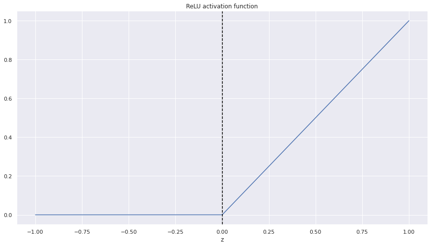
Thus, the activation function must be non-linear. The sigmoid function is non-linear, so it can be used as an activation function. But there are other options. Let me present you the Rectified Linear Unit (ReLU) function:
\[relu(z) = max\{0, z\}\]It may be easier if we plot it:

- If \(z <= 0\), the output is zero.
- If \(z > 0\), the output is the same as the input.
What is the advantage of the ReLU function versus the sigmoid? ReLU has mathematical properties that make the training process much faster. Concretely, it helps solve the vanishing gradient problem. If you are interested in this topic, this post explores it further.
Note that ReLU is not bounded: if \(z\) becomes arbitrarily large, the output will be as big as the input. If we are dealing with binary classification, this makes it inadequate for the output layer, as the output unit should produce a number \(y_{prob} \in [0, 1]\) that can be interpreted as a probability.
How do we solve this? We will make each layer have its own activation function:
- Hidden layers (layers 1 and 2, in our example) will use ReLU: \(g^{[1]}(z) = g^{[2]}(z) = relu(z)\).
- The output layer will keep using the sigmoid function: \(g^{[3]}(z) = \sigma(z)\).
Following this scheme, we will keep getting output probabilities in the valid range while making the training process faster!
Conclusion
That’s it for the basic of neural networks! We’ve covered what they are and how they make predictions. You know what hidden units, layers and activation functions are, which are the parameters of a network layer and how they are used to predict the outputs.
In the next post I will present the MNIST dataset and will explain how we can extend our neural network to handle multiclass classification.
I hope you enjoyed it! Feedback and suggestions are always welcome.
References
- Deep Learning Specialization, Coursera courses by Andrew Ng: https://www.coursera.org/specializations/deep-learning
- When not to use Neural Networks, by Rahul Bhatia: https://medium.com/datadriveninvestor/when-not-to-use-neural-networks-89fb50622429
- A Gentle Introduction to the Rectified Linear Unit (ReLU), by Jason Brownlee: https://machinelearningmastery.com/rectified-linear-activation-function-for-deep-learning-neural-networks/
- Sklearn documentation: https://scikit-learn.org/stable/
- XGBoost documentation: https://xgboost.readthedocs.io/en/latest/