Have you heard about Keras but never known what is it about or where to start with? In this post we will explain Keras basics and we will use it to build a handwritten digit classifier with a high level of accuracy! This is the last of a series of posts on neural networks. If you don’t know what terms like hidden unit or activation function mean, you may find it useful to read the first post of the series, on the basics of NNs. The problem presented here is a multiclass classification one, which the second post is all about.

TL; DR: code for this tutorial is here.

Problem statement

Imagine you’re working for the post service. Packets are routed using their postcode. You would like to come up with a model that knows how to read the handwritten numbers in the envelope postcodes, so you can automate the entire process. The problem of identifying a digit given an image is called handwritten digit recognition.

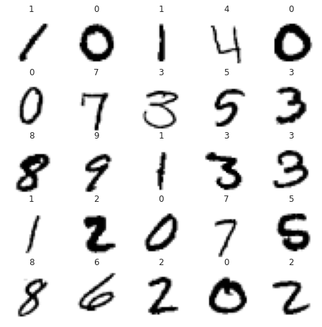
We will be working with the MNIST database of handwritten digits, which is the de-facto “hello world” dataset for computer vision applications. It consists of a set of 28 by 28 grayscale images containing handwritten digits. Each image is labeled from 0 to 9, according to the digit it represents. This is what the dataset looks like:

Our task is to build a model that classifies as much images correctly as it can. This is a multiclass classification problem, as there are 10 possible classes an image may belong to. We will be using accuracy to measure the classifier’s performance.

The MNIST dataset is available in Kaggle through this competition. I will show some code snippets throughout this post; you can find the entire code listing for it in this Kaggle kernel.

Network architecture

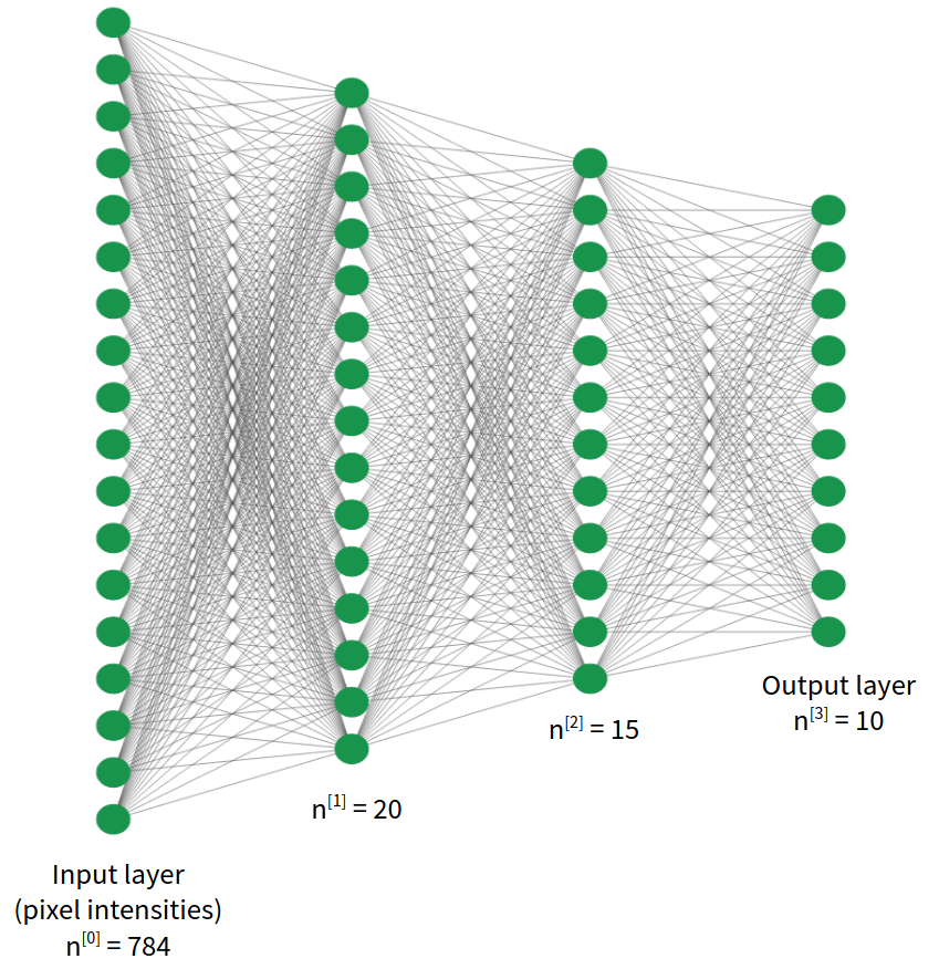
We will implement a fully connected neural network architecture like the one shown in the image.

Each image has \(\text{28 x 28} = 784\) grayscale pixel intensities. That means each image can be described as a set of 784 real numbers. We will simply use these as input features for our network. The output layer will have 10 units, as there are 10 possible classes in our classification problem, and will use the softmax activation function. The network will output a prediction vector \(y_{prob} \in \mathbb{R}^{10}\), each element representing the probability that the given image is a certain digit (e.g. \(y_{prob}[2]\) represents the probability that the input image is the digit 2). We will employ cross-entropy as the loss function. If you feel unsure about any of these concepts, feel free to check the previous post on neural networks for multiclass classification.

Keras and Tensorflow

Okay, we now know what we want to build. Let’s see how to build it. We will use the Keras framework, which makes it easy to define models like the one presented above.

If you’re familiar with the current deep learning landscape, you probably have heard both of Keras and Tensorflow. And you may be confused about the relationship between them: what is the difference between them? Is Keras part of Tensorflow? Does Keras use Tensorflow?

Keras is a library to build neural network models, and tries to be as simple as it can. On the other hand, Tensorflow is a symbolic math library which allows creating arbitrary machine learning models. Keras is higher level (and thus simpler) than Tensorflow. Actually, Keras uses Tensorflow. We will be using just Keras because our model is simple enough to be directly supported by the Keras APIs.

As of Keras 2.3.0, keras is included in the tensorflow Python package. This has not always been the case; if you are interested to know more about the history of these two libraries, check this post out.

With that in mind, let’s do the import:

1

from tensorflow import keras

When building a model with Keras, you should perform these three steps:

1. Defining the network architecture. This is writing in code the model architecture we explained before.
2. Compiling the model. At this point we specify the loss function, and other parameters of the training process, like the optimizer.
3. Fitting the model. Here we actually pass in the data so Keras can train the network.

We will go through them in the next sections.

Defining the architecture

We will be using the Sequential class, which is the easiest when we have a simple networks like ours. The model definition looks like the following:

1
2
3
4
5
6
7
8
9
10

lambda_ = 1e-2
model = keras.Sequential([
    keras.Input(shape=(784,)),
    keras.layers.Dense(20, activation='relu', name='l1',
    		           kernel_regularizer=keras.regularizers.l2(lambda_)),
    keras.layers.Dense(15, activation='relu', name='l2',
    		           kernel_regularizer=keras.regularizers.l2(lambda_)),
    keras.layers.Dense(10, activation='softmax', name='output',
    		           kernel_regularizer=keras.regularizers.l2(lambda_))
])

• The Sequential class takes as input a list of layers and connects them in sequential order. This class is a Keras Model, which means it offers operations like compile(), fit() and predict().
• The Input object represents the input layer. We pass in a tuple indicating the shape of the input feature vector. Remember that we have a feature per pixel, and that yields 784 features. Note that we do not have to specify how many samples we have.
• We use Dense objects to represent fully connected layers. The first parameter is the number of hidden units. The first two layers use the ReLU activation function, while the output layer uses softmax. The name parameter is optional and is used for display and debugging purposes only.
• We have included layer weight regularizers in all the layers. Regularization is a technique to prevent overfitting. The higher the lambda_ parameter, the stronger the regularizer effect is.

Note that the alternative to the sequential class is the functional API, which you can employ for more complex architectures.

Compiling the model

Let’s dive into the second step:

1
2
3
4
5

model.compile(
    optimizer=keras.optimizers.Adam(),
    loss='categorical_crossentropy',
    metrics=['accuracy']
)

This is telling Keras additional information about how to perform the training process:

• The Adam optimizer should be used. The optimizer is the algorithm that solves the minimization problem that training presents: given a labeled training set, it tries to find the set of weights that make the loss function as small as possible. You may have heard of gradient descent, as it is the most essential optimizer used in deep learning. Adam is a modified version of gradient descent that usually works better. This post explores the algorithm in depth.
• It should use the categorical cross-entropy loss function. Check the previous post if you are not familiar with this loss function.
• During the training process, Keras will track the accuracy metric. This means it will record the evolution of this score as the network is trained, both for training and validation data. By looking at this information we can get insights like if we are training the network long enough or not. You can track as many metrics as you want. A comprehensive list of available metrics is here.

Fitting the model

Finally, let’s tell Keras to train our network. Let’s say we have 42000 training examples:

1
2
3
4
5
6
7
8
9
10
11
12
13
14

X_train = # ... read input data; X_train.shape is (42000, 784)
labels =  # ... read input data; labels.shape is (42000, 1)
          #     and each value is between 0 and 9

# convert to one-hot, y_train.shape is (42000, 10)
y_train = keras.utils.to_categorical(labels) 

history = model.fit(
    X_train, 
    y_train, 
    validation_split=0.2,
    batch_size=128, 
    epochs=50
)

• We have converted our numeric labels to a one-hot encoding, using the to_categorical helper function. Recall that in this one-hot encoding scheme, every label is represented by a vector of 10 elements, one per possible class.
• validation_split=0.2 tells Keras to perform a train-validation split before fitting the data. Keras will use 80% of the training examples to actually train the network, leaving the remaining 20% out for validation, so we can have unbiased estimates of our metrics.
• batch_size sets the mini-batch size. Mini-batching is a technique that makes the optimization process quicker. The cost function is usually defined as the average over all the training set of the loss function. If you have a big training set, computing the cost function on the entire training set may be very expensive. Instead, optimization algorithms usually work in mini-batches: they first look into a small subset of the data and make some progress towards the minimum. They then jump into the next mini-batch, repeating the process until they pass through all the training set. This allows for faster progress. This article explores the topic of mini-batches for gradient descent, and is extrapolable to the Adam optimization algorithm.
• epochs controls how long the network should be trained for. An epoch is a pass of the optimization algorithm through the entire training set. Setting epochs=50 means that the algorithm will stop after 50 passes. You should specify a number of epochs big enough such that further training yields no significant gain in performance. We can use the tracked metrics to verify this.
• model.fit() returns a history object, containing the tracked metrics. We will explore it further in the next section.

Evaluating the model

By providing validation data with validation_split, Keras performs model validation for us while training. By looking at the logs, I’m getting 96.48% accuracy on the train set and a 94.63% on the validation set, which is quite good for a simple network like ours. Note that the decimals may vary for you due to random initialization of weights. Train and validation scores are quite close, so it doesn’t seem like our model is overfitting a lot.

Would our model improve if we trained it further? We can examine the returned history object to answer this question:

1
2
3
4

loss = history.history['loss']
val_loss = history.history['val_loss']
acc = history.history['accuracy']
val_acc = history.history['val_accuracy']

Note that:

• history is a keras.callbacks.History object.
• history.history is a Python dict containing the recorded values for the loss and each defined metric.
• Each of the four items are Python lists with an element per epoch. In our case, the lists contain 50 elements.
• loss is the value of the loss function for the training set; val_loss is the loss function for the validation set.
• The same applies for accuracy and val_accuracy.

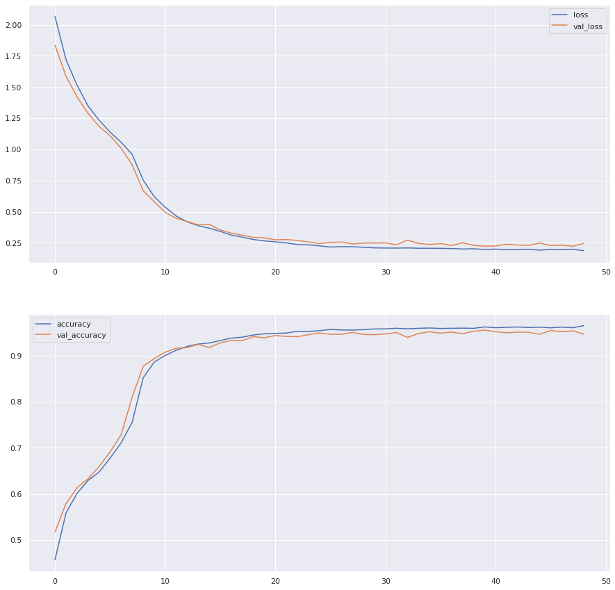
If we plot these measures against the epoch number, we get the following:

We can see that the loss goes down sharply at first and then flattens. The accuracy shows the reverse tendency. After 50 epochs, the performance seems almost flat. Thus, training the network longer won’t yield much better results. We can also see that both train and validation scores are quite close, which indicates we are not overfitting heavily.

Making predictions

You can make predictions for a bunch of examples:

1
2

preds_prob = model.predict(X_test)
preds_label = preds_prob.argmax(axis=1)

Where X_test has the same columns as X_train. predict() returns an array of probabilities, with 10 columns, one for each class. We can transform that into a label using numpy’s argmax in each row (axis=1).

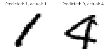
Finally, let’s inspect both a correct and a wrong prediction:

Conclusion

This concludes our three-post series on neural networks! Thanks for reading this far. As always, please share, and feedback is always welcome!

References

• Deep Learning Specialization, Coursera courses by Andrew Ng: https://www.coursera.org/specializations/deep-learning.
• How to attack a machine learning model?, Kaggle kernel by Laura Fink: https://www.kaggle.com/allunia/how-to-attack-a-machine-learning-model.
• Digit Recognizer, Kaggle competition: https://www.kaggle.com/c/digit-recognizer.
• NN-SVG, a tool to draw neural network architectures by Alexander Lenail: http://alexlenail.me/NN-SVG/index.html.
• Keras vs. tf.keras: What’s the difference in TensorFlow 2.0?, by Adrian Rosebrock: https://www.pyimagesearch.com/2019/10/21/keras-vs-tf-keras-whats-the-difference-in-tensorflow-2-0/
• Regularization in Machine Learning, by Prashant Gupta: https://towardsdatascience.com/regularization-in-machine-learning-76441ddcf99a.
• Gentle Introduction to the Adam Optimization Algorithm for Deep Learning, by Jason Brownlee: https://machinelearningmastery.com/adam-optimization-algorithm-for-deep-learning/.
• Batch, Mini Batch & Stochastic Gradient Descent, by Sushant Patrikar: https://towardsdatascience.com/batch-mini-batch-stochastic-gradient-descent-7a62ecba642a.
• Keras official documentation: https://keras.io/.